Watch \(\mathbf{w}\) and \(b\) move from \((0, 0, 0)\) toward a separating boundary on AND by hand. Then watch the same arithmetic rotate forever on XOR. Same rule; different fate, because the data shape differs — not the algorithm.
Update rule, applied per sample \((\mathbf{x}_i, y_i)\):
\[
\text{if } y_i(\mathbf{w}^\top\mathbf{x}_i + b) \le 0:\quad
\mathbf{w} \mathrel{+}= y_i \mathbf{x}_i,\quad b \mathrel{+}= y_i
\]
30.2 AND: converges
Labels \(y = (-1, -1, -1, +1)\).
30.2.1 Epoch 1
Sample
\(y\)
\(\mathbf{w}^\top\mathbf{x}+b\)
\(y(\mathbf{w}^\top\mathbf{x}+b)\)
Mistake?
New \(\mathbf{w}\)
New \(b\)
(0,0)
−1
0
0
yes
(0,0)
−1
(0,1)
−1
−1
1
no
(0,0)
−1
(1,0)
−1
−1
1
no
(0,0)
−1
(1,1)
+1
−1
−1
yes
(1,1)
0
30.2.2 Epoch 2
Sample
\(y\)
\(\mathbf{w}^\top\mathbf{x}+b\)
\(y(\mathbf{w}^\top\mathbf{x}+b)\)
Mistake?
New \(\mathbf{w}\)
New \(b\)
(0,0)
−1
0
0
yes
(1,1)
−1
(0,1)
−1
0
0
yes
(1,0)
−2
(1,0)
−1
−1
1
no
(1,0)
−2
(1,1)
+1
−1
−1
yes
(2,1)
−1
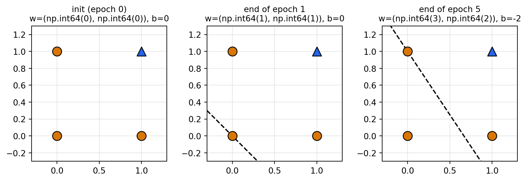
By epoch ~5 the rule settles into a separator that classifies all four corners correctly. The figure below visualizes the boundary at three checkpoints.
Code
import numpy as np, matplotlib.pyplot as pltX = np.array([[0,0],[0,1],[1,0],[1,1]], dtype=float)y = np.array([-1,-1,-1,+1])w = np.zeros(2); b =0.0snapshots = {"init (epoch 0)": (w.copy(), b)}for epoch inrange(1, 6):for xi, yi inzip(X, y):if yi * (w @ xi + b) <=0: w += yi * xi b += yiif epoch in (1, 5): snapshots[f"end of epoch {epoch}"] = (w.copy(), b)fig, axes = plt.subplots(1, 3, figsize=(9, 3))for ax, (title, (ww, bb)) inzip(axes, snapshots.items()):for xi, yi inzip(X, y): c ="#d97706"if yi <0else"#2563eb" m ="o"if yi <0else"^" ax.scatter(*xi, c=c, marker=m, s=120, edgecolor="k", zorder=3)ifabs(ww[1]) >1e-9: xs = np.array([-0.3, 1.3]) ys =-(ww[0]*xs + bb) / ww[1] ax.plot(xs, ys, "k--", lw=1.5) ax.set_xlim(-0.3, 1.3); ax.set_ylim(-0.3, 1.3) ax.set_aspect("equal"); ax.grid(alpha=0.3) ax.set_title(f"{title}\nw={tuple(ww.astype(int))}, b={int(bb)}", fontsize=10)plt.tight_layout(); plt.show()
Orange circles are negatives; blue triangles are the single positive. The dashed line \(\mathbf{w}^\top\mathbf{x} + b = 0\) rotates toward the misclassified positive and away from misclassified negatives, until it lands on a side of the unit square that puts (1,1) alone above and the other three below.
30.3 XOR: never converges
Same \(X\), but labels \(y = (-1, +1, +1, -1)\) — the diagonals are positive, the antidiagonals are negative.
30.3.1 Epoch 1
Sample
\(y\)
\(\mathbf{w}^\top\mathbf{x}+b\)
\(y(\mathbf{w}^\top\mathbf{x}+b)\)
Mistake?
New \(\mathbf{w}\)
New \(b\)
(0,0)
−1
0
0
yes
(0,0)
−1
(0,1)
+1
−1
−1
yes
(0,1)
0
(1,0)
+1
0
0
yes
(1,1)
1
(1,1)
−1
3
−3
yes
(0,0)
0
After four mistakes in one epoch, \((\mathbf{w}, b)\) has returned to \((0, 0, 0)\). Subsequent epochs repeat the cycle indefinitely.
The geometry tells the same story: no straight line through the unit square can put (0,0) and (1,1) on one side while putting (0,1) and (1,0) on the other.
30.4 What this table teaches
The rule updates only on mistakes. Correctly classified samples leave \(\mathbf{w}, b\) untouched.
The boundary rotates predictably: toward misclassified positives, away from misclassified negatives.
Convergence depends on the data, not the algorithm. Linearly separable data → finite mistake count (Novikoff bound). Non-separable data → indefinite oscillation, often cyclic.
The arithmetic is concrete and small. Every step is an addition or comparison on a 2-dimensional vector. The “mystery” of learning, in this case, is just bookkeeping.