Backprop gives the gradient; optimization is the update rule applied to it. Walk downhill — \(\boldsymbol{\theta} \leftarrow \boldsymbol{\theta} - \eta\,\nabla\mathcal{L}\). SGD estimates that gradient on a cheap, noisy mini-batch; momentum accumulates a velocity to accelerate along consistent directions and damp oscillation. Adaptive optimizers (Adam) build on exactly this, later.
Backprop (chapter 04) computes \(\nabla\mathcal{L}\); it does not say how to use it. Optimization is the update machinery — and it is a direct descendant of the perceptron’s rule from chapter 01. The perceptron nudged \(\mathbf{w}\) on each mistake; gradient descent generalizes that to any differentiable loss, and SGD + momentum make it fast and stable enough to train large networks. The choice of optimizer sets training speed, stability, and often the quality of the final solution.
8.2 The mechanism
8.2.1 Gradient descent
The basic rule moves parameters opposite the gradient (Cauchy, 1847):
The learning rate\(\eta\) is the one knob that matters most: too large and the iterates diverge or oscillate; too small and training crawls. Batch GD uses the full dataset for each step — accurate, but expensive.
8.2.2 Stochastic gradient descent
SGD replaces the full-dataset gradient with an estimate from a mini-batch(Robbins & Monro, 1951):
It is far cheaper per step, and the noise is often a feature, not a bug: it helps escape saddle points and sharp minima. Essentially all deep-network training is mini-batch SGD or a descendant.
8.2.3 Momentum
Plain GD crawls along gently sloped directions and oscillates across steep ones (the ill-conditioned bowl from chapter 05). Momentum(Polyak, 1964) accumulates a velocity, so consistent gradient directions build speed while oscillations cancel:
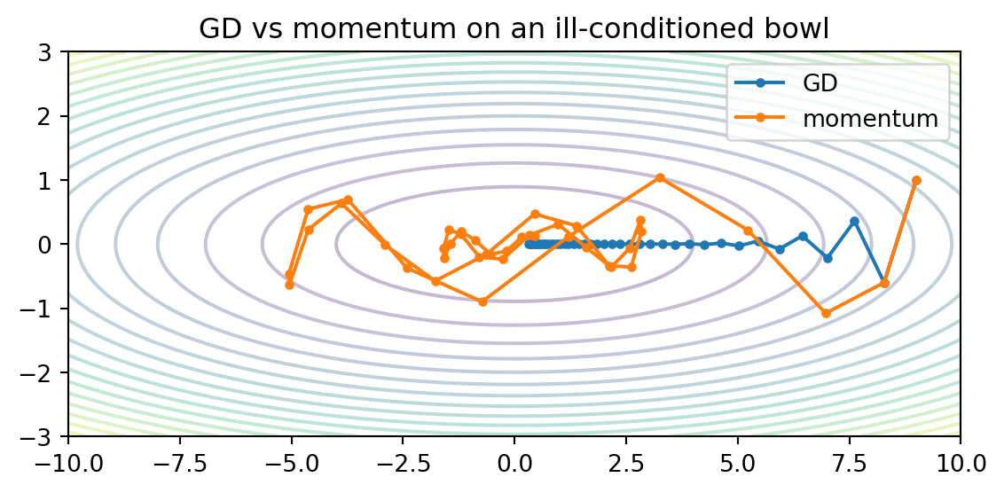
On an ill-conditioned quadratic (steep in one axis, shallow in the other), watch momentum damp the oscillation and converge faster.
import numpy as np, matplotlib.pyplot as plta, b =1.0, 20.0# curvatures: shallow x, steep ygrad =lambda p: np.array([a*p[0], b*p[1]])def run(kind, steps=40, lr=0.08, beta=0.9): p = np.array([9.0, 1.0]); v = np.zeros(2); traj = [p.copy()]for _ inrange(steps): g = grad(p)if kind =="gd": p = p - lr*gelse: v = beta*v + g p = p - lr*v traj.append(p.copy())return np.array(traj)gd, mom = run("gd"), run("momentum")xs, ys = np.linspace(-10, 10, 100), np.linspace(-3, 3, 100)Xg, Yg = np.meshgrid(xs, ys); Z =0.5*(a*Xg**2+ b*Yg**2)plt.figure(figsize=(6, 3))plt.contour(Xg, Yg, Z, levels=20, alpha=0.3)plt.plot(gd[:,0], gd[:,1], "o-", ms=3, label="GD")plt.plot(mom[:,0], mom[:,1], "o-", ms=3, label="momentum")plt.legend(); plt.title("GD vs momentum on an ill-conditioned bowl")plt.tight_layout(); plt.show()
8.2.5 What to observe
GD zig-zags across the steep axis and inches along the shallow one — the classic ill-conditioning slowdown.
Momentum cancels the back-and-forth (opposing steps subtract in the velocity) and builds speed down the shallow axis — reaching the minimum in far fewer steps.
Neither changes the gradient itself; they change how the gradient is used. That is the whole job of an optimizer.
WarningPitfall: the learning rate dominates
Most training failures are learning-rate failures: too high → divergence or NaN; too low → apparent plateaus mistaken for convergence. Momentum adds a second knob (\(\beta\)) that can overshoot if set too high. Tune \(\eta\) first; schedules and adaptive methods (later) automate part of this.
8.3 Application & impact
This machinery is live, not legacy — every network in this book is trained by a descendant of SGD.
optimizer.step() in PyTorch is this update; SGD(momentum=0.9) is literally the Polyak rule above.
AdamW, which trains most modern LLMs, is momentum plus a per-parameter adaptive learning rate — a direct extension of what’s here, detailed in Adaptive Optimizers.
The XOR demo in chapter 04 was already doing this — plain gradient descent on the cross-entropy loss.
NoteKey takeaway
Optimization turns gradients into learning. Gradient descent is the skeleton, SGD makes it affordable, momentum makes it fast — and every adaptive optimizer later in the timeline is a refinement of these three moves, not a replacement.
Robbins, H., & Monro, S. (1951). A stochastic approximation method. The Annals of Mathematical Statistics, 22(3), 400–407. https://doi.org/10.1214/aoms/1177729586
Polyak, B. T. (1964). Some methods of speeding up the convergence of iteration methods. USSR Computational Mathematics and Mathematical Physics, 4(5), 1–17. https://doi.org/10.1016/0041-5553(64)90137-5