A learning signal answers “how wrong, and how confidently?” — not just “right or wrong?”. Cross-entropy measures the cost of a probabilistic prediction \(q\) against a true label \(p\): \[H(p, q) = -\sum_x p(x)\log q(x).\] It is the loss behind nearly every classifier and language model. The math is Shannon’s, from 1948 — a decade before the perceptron’s update rule.
The perceptron’s update rule reacts to a 0/1 mistake: right or wrong, nothing in between. That signal has no gradient — you cannot ask “how much should I change \(\mathbf{w}\) to be a little less wrong?” Every method after the perceptron trains by gradient descent on a smooth loss, which means a differentiable measure of how wrong a probabilistic prediction is. That measure is cross-entropy, and its foundations were laid by Shannon (Shannon, 1948) in 1948 — chronologically before the perceptron, which is why it sits here, early in the timeline.
The treatment here focuses on binary classification (the perceptron’s own domain). The multi-class generalization (softmax + categorical cross-entropy) is introduced later, where multi-output models first appear — the language-model output head in Output Layer & Decoding.
4.2 The mechanism
4.2.1 Surprise and entropy
Shannon’s self-information of an event with probability \(p\) is \(-\log p\): rare events are surprising, certain events (\(p = 1\)) carry zero surprise. Entropy is the expected surprise of a distribution:
\[
H(p) = -\sum_x p(x) \log p(x).
\]
For a binary outcome with \(P(\text{1}) = p\), entropy peaks at \(p = 0.5\) (maximum uncertainty) and is zero at \(p \in \{0, 1\}\) (no uncertainty).
4.2.2 Cross-entropy
If the true distribution is \(p\) but the model predicts \(q\), the expected cost of encoding outcomes with \(q\) is the cross-entropy:
\[
H(p, q) = -\sum_x p(x) \log q(x).
\]
It is minimized, for fixed \(p\), exactly when \(q = p\). As a training loss, \(p\) is the (known) label distribution and \(q\) is the model’s prediction.
4.2.3 Binary cross-entropy
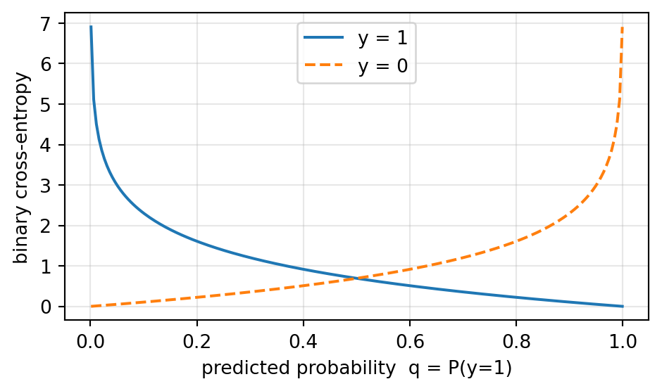
For a label \(y \in \{0, 1\}\) and a model prediction \(q = P(y = 1)\), the true distribution puts all mass on the observed label, so the sum collapses to a single, clean expression:
A confident-correct prediction (\(q \to 1\) when \(y = 1\)) drives the loss to \(0\); a confident-wrong one (\(q \to 0\) when \(y = 1\)) drives it to \(+\infty\). That asymmetry — gentle on correct, brutal on confidently wrong — is what makes the gradient informative.
4.2.4 KL divergence
The gap between cross-entropy and the irreducible entropy of \(p\) is the Kullback–Leibler divergence(Kullback & Leibler, 1951):
Since \(H(p)\) is fixed by the data, minimizing cross-entropy is exactly minimizing \(D_{\mathrm{KL}}(p\,\|\,q)\) — pushing the model’s distribution toward the data’s. (And minimizing cross-entropy is equivalent to maximizing log-likelihood — the same objective from a statistician’s chair. If maximum-likelihood estimation is unfamiliar, the Prerequisites appendix has a one-table refresher.)
4.2.5 Minimal sketch
import numpy as npdef bce(y, q, eps=1e-12): q = np.clip(q, eps, 1- eps) # guard against log(0)return-(y*np.log(q) + (1-y)*np.log(1-q))# A positive example (y=1) under increasingly confident predictions:for q in [0.5, 0.7, 0.9, 0.99, 0.01]:print(f"y=1, q={q:>4}: BCE = {bce(1, q):.4f}")
BCE is smooth and differentiable everywhere in \((0, 1)\) — unlike the perceptron’s 0/1 mistake count, it gives a gradient at every prediction.
It is unbounded: a confidently wrong prediction is penalized without limit, which strongly discourages overconfidence.
At \(q = 0.5\) the loss is \(\log 2 \approx 0.693\) — the “I don’t know” baseline for one bit.
WarningPitfall: loss is not accuracy
Cross-entropy and accuracy measure different things. A model can improve its loss (becoming better-calibrated, less overconfident) while its accuracy is unchanged, and vice versa. Train on cross-entropy because it has useful gradients; report accuracy (or BLEU, perplexity, …) because it’s what you actually care about.
4.3 Application & impact
Cross-entropy is not legacy — it is the live training objective for essentially every classifier and language model in 2026.
4.3.1 What this becomes
Concept here
What it becomes
Where you see it today
Binary cross-entropy
Categorical cross-entropy (softmax over \(K\) classes)
Every multi-class classifier; introduced later in the timeline
Cross-entropy over a vocabulary
Next-token prediction loss
The pretraining objective of every LLM
\(\exp(\text{cross-entropy})\)
Perplexity
The standard language-model metric
KL divergence
Regularizer / distance between distributions
VAEs, knowledge distillation, the KL penalty in RLHF, DPO
CE = \(-\log\)-likelihood
Maximum-likelihood estimation
The probabilistic justification for the whole setup
4.3.2 Concretely, where the lineage lands
Logistic regression trains a single neuron with exactly the BCE above — it is the perceptron with a probability output and a differentiable loss.
A language model computes cross-entropy between its predicted next-token distribution and the one-hot true token, summed over a sequence. Scaling that is the entire pretraining objective.
RLHF / DPO add a KL term to keep a fine-tuned policy close to a reference model — the same \(D_{\mathrm{KL}}\) defined above.
NoteKey takeaway
Going from a 0/1 mistake to a probabilistic cross-entropy is what makes gradient-based learning possible. Shannon handed us the measure in 1948; the rest of the timeline is, in large part, minimizing cross-entropy with ever-larger models.
Kullback, S., & Leibler, R. A. (1951). On information and sufficiency. The Annals of Mathematical Statistics, 22(1), 79–86. https://doi.org/10.1214/aoms/1177729694