Backprop multiplies one factor per layer. In a deep stack those factors compound: if each is \(< 1\) the gradient vanishes exponentially; if \(> 1\) it explodes. \[\|\boldsymbol{\delta}^{(1)}\| \sim \prod_{l} \|\mathbf{W}^{(l)}\|\,\big|\phi'(\mathbf{z}^{(l)})\big|.\] This single fact — identified by Hochreiter (1991) and Bengio et al. (1994) — is the central obstacle to depth, and the reason much of the rest of this timeline exists.
The previous chapter gave the backward recursion. This one asks: what happens to that signal across many layers? The answer is the deepest practical problem in the field’s history. Because backprop multiplies a weight-and-derivative factor at every layer, the gradient reaching early layers is a long product. Products of numbers below one collapse toward zero; products above one blow up. Either way, early layers get an unusable signal — vanishing or exploding gradients (Bengio et al., 1994; Hochreiter, 1991).
This is not a minor caveat. It is why deep sigmoid/tanh networks were nearly untrainable for years, why vanilla RNNs cannot learn long-range dependencies, and the direct motivation for LSTM gating, residual connections, normalization, and non-saturating activations — most of the architectural story still to come.
The behavior is governed by whether the typical factor is below or above 1:
Vanishing: factor \(< 1\) → \(\|\boldsymbol{\delta}^{(1)}\|\) decays like \(r^{L}\), \(r<1\). With sigmoid (\(\phi' \le 0.25\)), decay is severe.
Exploding: factor \(> 1\) (large weights) → growth like \(r^{L}\), \(r>1\), producing NaN losses (Pascanu et al., 2013).
7.2.2 Minimal sketch: gradient norm across depth
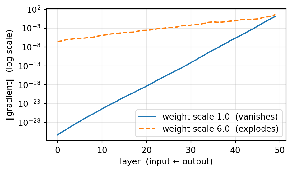
Propagate an error signal back through a 50-layer sigmoid stack and watch its norm on a log scale.
import numpy as np, matplotlib.pyplot as pltrng = np.random.default_rng(0)L, dim =50, 32sig =lambda z: 1/ (1+ np.exp(-z))def gradient_norms(weight_scale): Ws = [rng.normal(size=(dim, dim)) * weight_scale / np.sqrt(dim) for _ inrange(L)] a = rng.normal(size=dim); acts = [a]for W in Ws: # forward a = sig(W @ a); acts.append(a) delta = rng.normal(size=dim) # error injected at the output norms = []for l inreversed(range(L)): # backward delta = (Ws[l].T @ delta) * acts[l+1] * (1- acts[l+1]) norms.append(np.linalg.norm(delta))return norms[::-1]plt.figure(figsize=(5, 3))plt.semilogy(gradient_norms(1.0), label="weight scale 1.0 (vanishes)")plt.semilogy(gradient_norms(6.0), "--", label="weight scale 6.0 (explodes)")plt.xlabel("layer (input ← output)"); plt.ylabel("‖gradient‖ (log scale)")plt.legend(); plt.grid(alpha=0.3); plt.tight_layout(); plt.show()
7.2.3 What to observe
On a log scale both curves are roughly straight lines — the hallmark of exponential behavior in depth.
The default-scale sigmoid stack vanishes: by layer 1 the gradient is many orders of magnitude smaller than at the output. Early layers barely learn.
Large weights explode in the opposite direction. The knife-edge between them is what good initialization targets — keeping the per-layer factor near 1 (Xavier/He; a look-ahead) (Glorot & Bengio, 2010).
WarningPitfall: depth alone is not progress
Stacking more layers does not monotonically help if gradients vanish: the early layers stop receiving signal and the effective depth is far less than the nominal depth. Naively going deeper without addressing gradient flow (init, normalization, residuals, gating) often makes training worse.
7.3 Application & impact
The vanishing/exploding gradient problem is arguably the most consequential entry in this book: a remarkable share of architectural innovation is, at heart, a fix for it.
7.3.1 What this problem motivated
The fix
What it does about gradient flow
Where in the timeline
LSTM / GRU gating
A near-additive cell path keeps the factor \(\approx 1\) (constant error carousel)
RNN era — the next part
ReLU & non-saturating activations
\(\phi' = 1\) for active units → no \(0.25\) shrink
deep-net / transformer era (deferred)
Careful initialization (Xavier/He)
Sets weight scale so the per-layer factor starts near 1
upcoming sidecar
Normalization (Batch/Layer/RMS)
Re-centers activations to avoid saturation each layer
transformer era
Residual connections
An identity path gives gradients a factor-1 shortcut
The LSTM (next part) exists primarily to solve this: its cell state is an additive path, so the gradient does not get multiplied into oblivion across time steps.
Residual connections in transformers are the same idea for depth: add, don’t only multiply, so a factor-1 route always exists.
Every modern stack combines several of these fixes at once — non-saturating activations + normalization + residuals + good init — which together is what finally made very deep networks routinely trainable.
NoteKey takeaway
Backprop’s strength — multiplying a factor per layer — is also its weakness: those factors compound into vanishing or exploding gradients. Hold this picture; the architectures ahead (LSTM gating, residuals, normalization) are best understood as different answers to “how to keep the per-layer factor near 1?”
Hochreiter, S. (1991). Untersuchungen zu dynamischen neuronalen netzen [PhD thesis]. Technische Universität München.
Bengio, Y., Simard, P., & Frasconi, P. (1994). Learning long-term dependencies with gradient descent is difficult. IEEE Transactions on Neural Networks, 5(2), 157–166. https://doi.org/10.1109/72.279181
Glorot, X., & Bengio, Y. (2010). Understanding the difficulty of training deep feedforward neural networks. Proceedings of the 13th International Conference on Artificial Intelligence and Statistics (AISTATS), 249–256.
Pascanu, R., Mikolov, T., & Bengio, Y. (2013). On the difficulty of training recurrent neural networks. Proceedings of the 30th International Conference on Machine Learning (ICML), 1310–1318.